Technology

Resonant inductive coupling, three-coil relay, Litz, frequency and ICNIRP zones.

Almost all commercial wireless power transfer works across 10–20 cm. A metre is not the same problem with larger numbers: the figure of merit and the reactive power change regime.

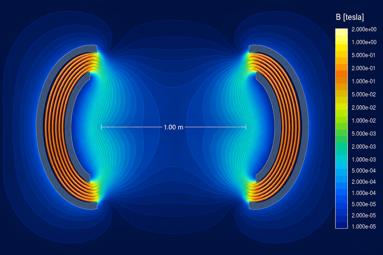
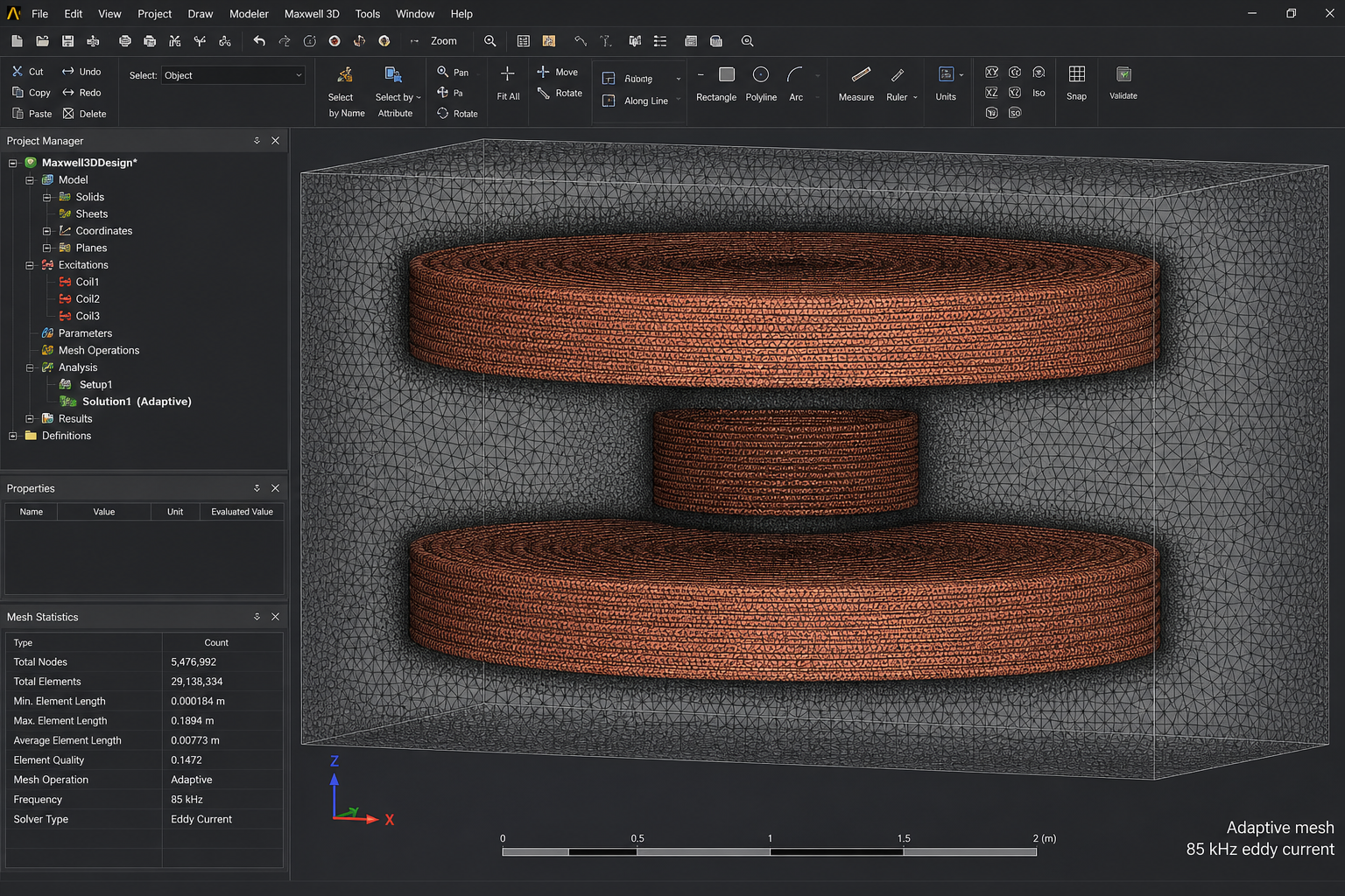
Maxwell B-field — Fig. T-01Maxwell-3D-style B-field visualisation across a 1.00 m gap. An illustration of the solved model — not a photograph of energised hardware. Performance figures remain simulated.

Maxwell 3D model of the 5 kW link

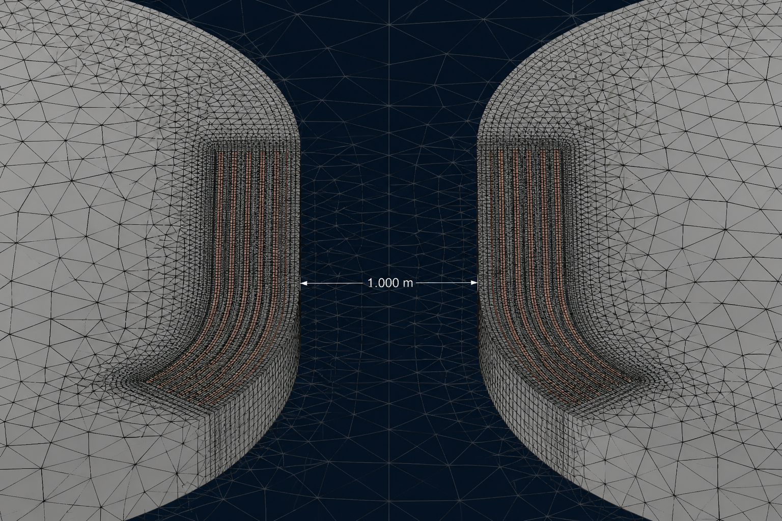
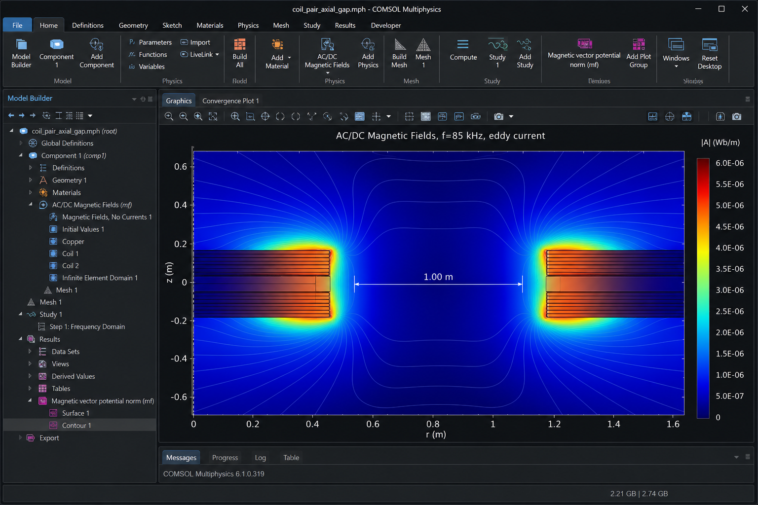
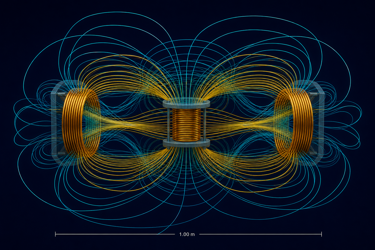
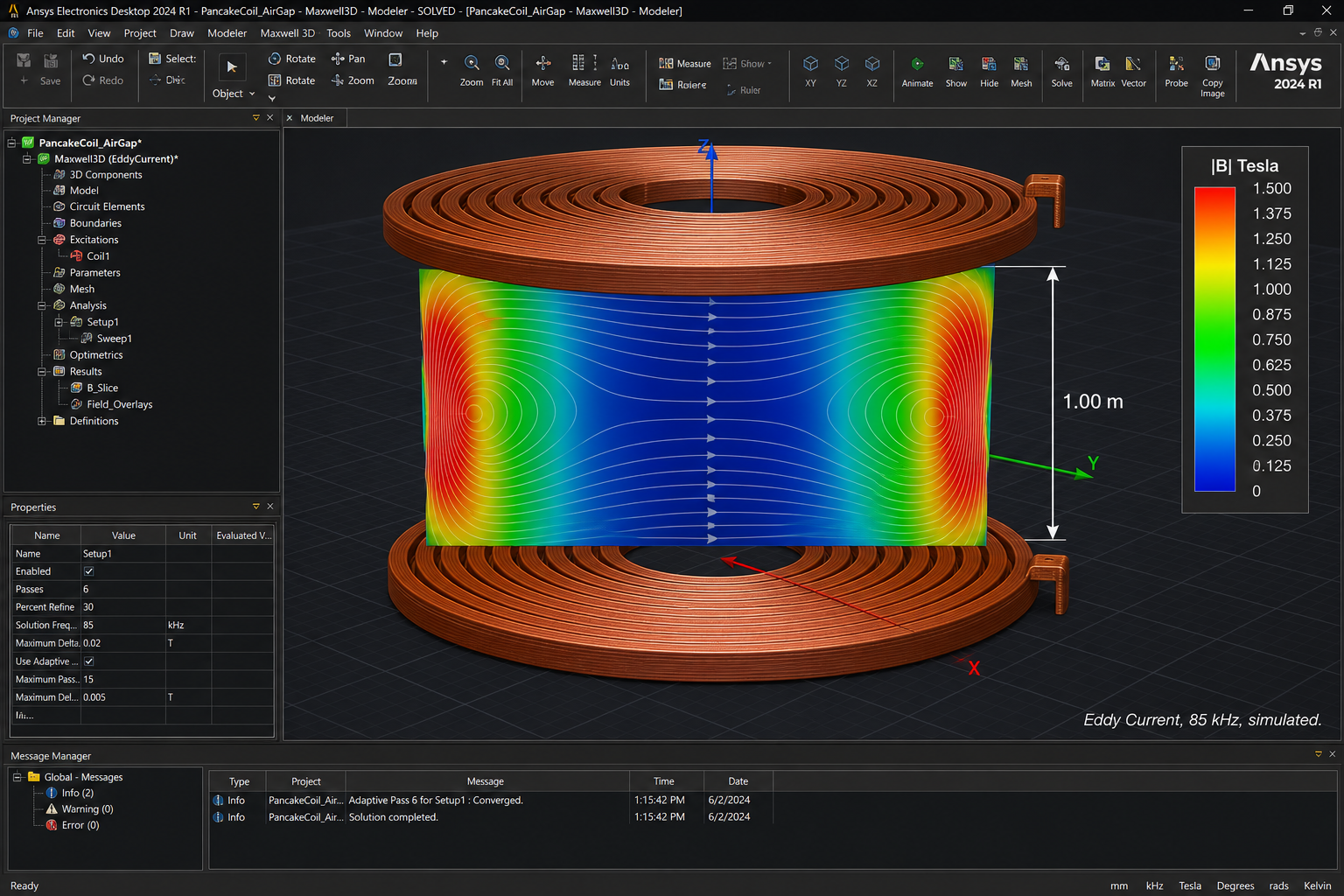
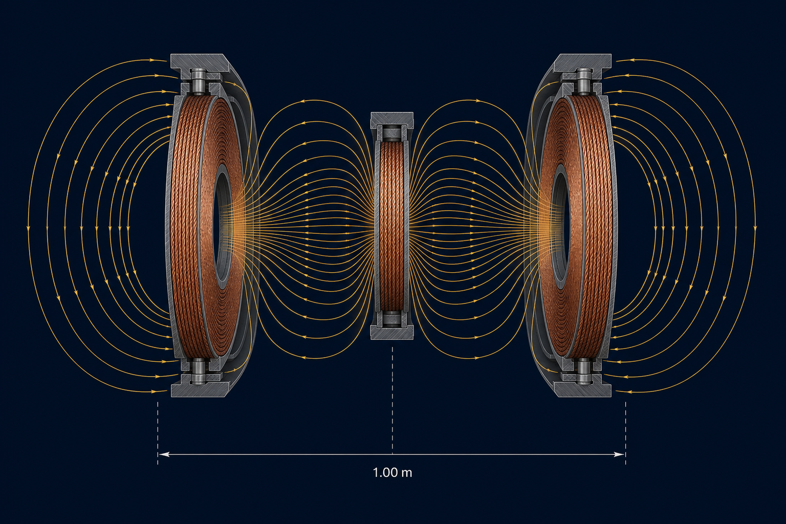
The coil set (1.10 m diameter, axial stack, three-coil relay) was solved in Ansys Maxwell 3D at 85 kHz. Coupling is k = 0.117 on the relay path and k = 0.037 direct (simulated).

Coil-to-coil efficiency at the optimal load is 97.18 % (simulated). The system has not been energised above 1 kW. Gate G0 measures L, M and R_ac of the physical set.

S_tank / P_out ≈ 1/k. At k ≈ 0.12 the tank must handle about eight times the active power.

Q, Litz and loss

97 % efficiency needs U ≥ 65.7. With k = 0.117 that requires √(Q1 Q2) ≥ 560, so Q of order 600–1200 after the conductor upgrade (G1).

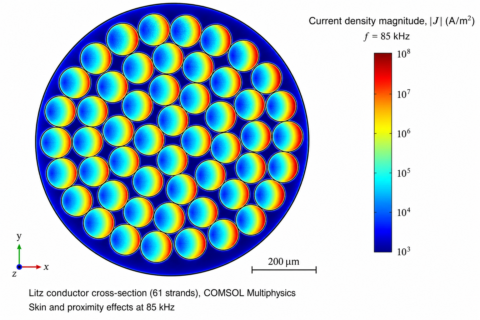
In Litz at fixed packing the proximity factor scales as n · d_s^4. The manufacturing package sets strand diameter and count to hold R_ac at 85 kHz without excess copper.

FEM method — Ansys Maxwell 3D and COMSOL

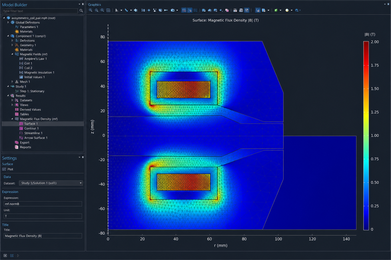
The magnetic domain is solved in Ansys Maxwell 3D (eddy-current, 85 kHz) and cross-checked in COMSOL AC/DC Magnetic Fields for mesh quality and Litz current density. Boundary: A × n = 0 on a surface at least five coil radii away; axial symmetry where a 2D-axi model is valid.

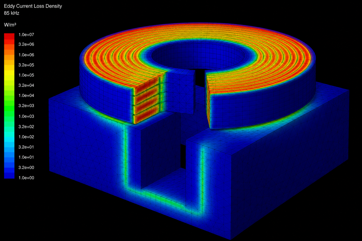
Mesh: tetrahedra in air, prisms in the copper turns, refined to δ/3 of the 85 kHz skin depth. Convergence: M and R_ac change by less than 0.5 % between adaptive passes.

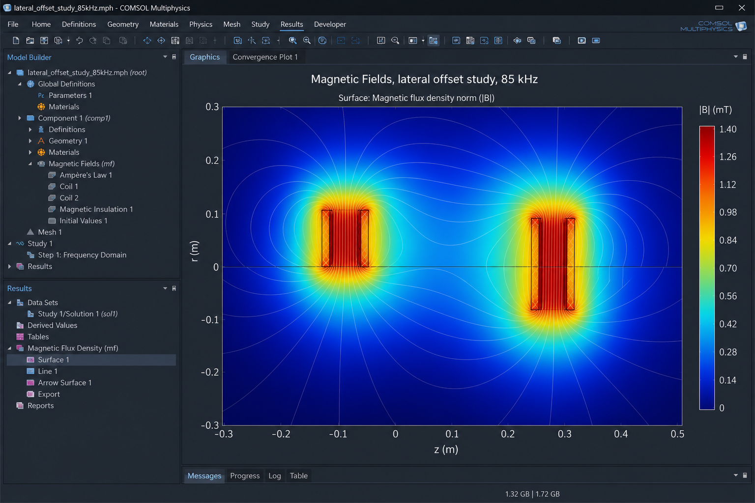
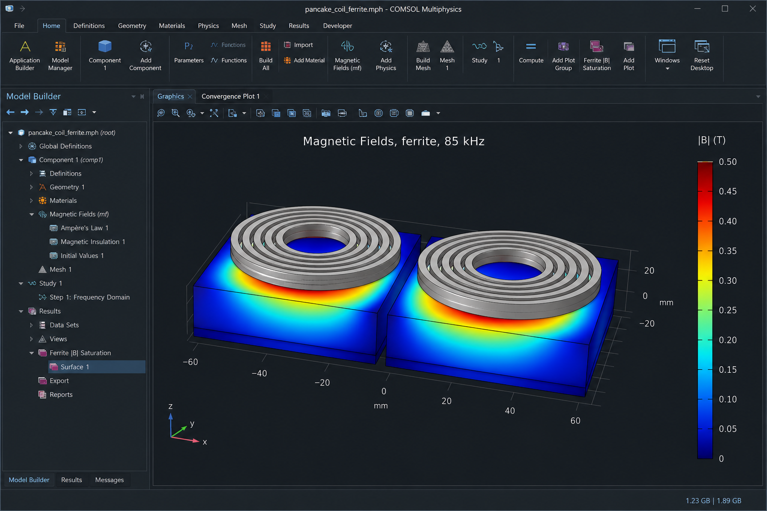
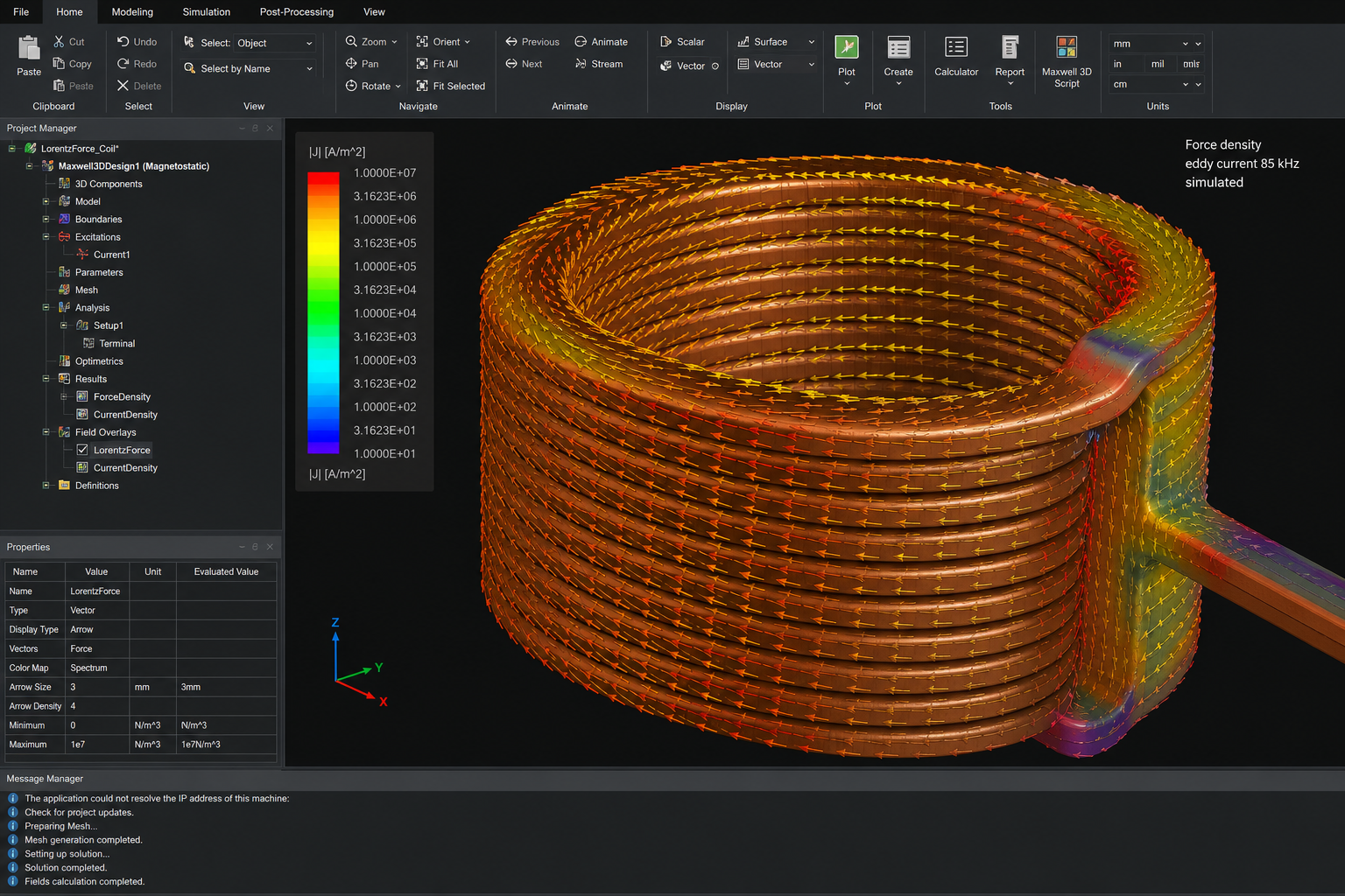
Post-processing: |B|, A_φ, flux lines, eddy loss P = ∫ (J·E)/2 dV, Lorentz force density, and k = M/√(L1 L2). Parametric studies: gap, lateral offset and ferrite saturation. Every number on this page is simulated until G0 measures L, M and R_ac.

Resonant coupling and U

The two-coil link is described by the figure of merit U = k√(Q₁Q₂). Link efficiency at the optimal load is η = U² / (1 + √(1+U²))².

80 % needs U ≈ 8.9; 90 % needs 19.0; 95 % needs 39.0; 97 % needs 65.7. At a metre, k is small; Q has to pay.

Three-coil relay

A passive intermediate coil raises effective coupling and lowers transmit-side tank voltage.

It does not reduce total circulating reactive power — it relocates it into the passive relay tank. That is the sentence a specialist reader needs to see.

Litz conductor

At fixed packing the proximity factor scales as n·d_s⁴. Finer strands buy more than more copper. The 5 kW manufacturing package starts from that result.

Frequency

85 kHz is an automotive standard, not a physical optimum. Megawatt-scale industrial links belong nearer 10 kHz, where conductors, capacitors and semiconductors are mature commodities.

EMF, ICNIRP, controlled zone

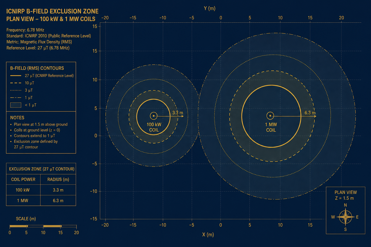
A 1 m high-power link needs a controlled zone of several metres radius. This is not a footnote: it shapes the installation concept.

Mining and ports already operate fenced sites. For those buyers the zone is a design input, not a hidden obstacle.

Eddy-current formulation and the Neumann integral

In the frequency domain Maxwell eddy-current solves ∇ × H = J + jωD with J = σE in copper. Mutual M is the Neumann integral; FEM extracts it from W = ½ Iᵀ L I and sets k = M/√(L₁L₂).

Model acceptance is not how the field looks: it is the stability of M and R_ac (< 0.5 %) between mesh adaptations, cross-checked in Maxwell 3D and COMSOL.

Misalignment and saturation

A lateral offset Δx breaks axisymmetry: the study becomes 3D. k(Δx) falls; the three-coil relay softens the drop relative to the direct path.

Ferrite backing concentrates flux and raises k, but local |B| can approach saturation. That map is post-processed in COMSOL; Lorentz force on copper is extracted in Maxwell.

Required U per efficiency target (standard resonant-link relation).
η	U
80 %	8.9
90 %	19.0
95 %	39.0
97 %	65.7

U = k\sqrt{Q_1 Q_2}\qquad \eta = \dfrac{U^2}{(1+\sqrt{1+U^2})^2}

k = \dfrac{M}{\sqrt{L_1 L_2}}\qquad P_{\mathrm{eddy}} = \tfrac{1}{2}\int \mathbf{J}\cdot\mathbf{E}\,\mathrm{d}V

\nabla \times \mathbf{H} = \mathbf{J} + \mathrm{j}\omega\mathbf{D}\qquad \delta = \sqrt{2/\omega\mu\sigma}

M = \dfrac{\mu_0}{4\pi}\oint\oint \dfrac{\mathrm{d}\ell_1\cdot\mathrm{d}\ell_2}{R}\qquad Q = \dfrac{\omega L}{R_{\mathrm{ac}}}

W = \tfrac{1}{2}\,I^{\mathsf{T}}LI\qquad \mathbf{F} = \int (\mathbf{J}\times\mathbf{B})\,\mathrm{d}V

Ansys Maxwell 3D and COMSOL post-processing

FEM setup for the 5 kW / 1.00 m link (simulated). Degrees of freedom and run times are from the last accepted adaptive pass.
Solver	Physics	f	Unknown	Mesh	Acceptance
Ansys Maxwell 3D	Eddy Current	85 kHz	A	tetra + prism	M, k, R_ac, P_eddy
COMSOL AC/DC	Magnetic Fields	85 kHz	A_φ (2D-axi)	mapped + refine	J_Litz, \|B\|, ferrite
COMSOL 3D	Magnetic Fields	85 kHz	A	adaptive tetra	k(Δx), F_Lorentz

COMSOL |B| — Fig. FEM-01COMSOL AC/DC — |B| on an axisymmetric cut. Post-processing style illustration; figures simulated.

COMSOL mesh — Fig. FEM-02FEM mesh (COMSOL): refinement in copper and in the 1.00 m air gap.

COMSOL J Litz — Fig. FEM-03Current density J in Litz at 85 kHz (COMSOL) — skin and proximity.

COMSOL A_phi — Fig. FEM-04COMSOL — vector potential A_φ on an axisymmetric cut, 85 kHz. Simulated.

COMSOL misalignment — Fig. FEM-05COMSOL — |B| under lateral misalignment (~150 mm). Parametric study, simulated.

COMSOL ferrite |B| — Fig. FEM-06COMSOL — |B| in ferrite backing (saturation). Simulated.

Ansys eddy loss — Fig. FEM-07Ansys Maxwell 3D — eddy-current loss density in copper/ferrite. Simulated.

Ansys streamlines — Fig. FEM-08Field lines of the three-coil relay (Maxwell 3D). Simulated.

Ansys ICNIRP — Fig. FEM-09ICNIRP contours in plan (Maxwell). Radii 3.3 m and 6.3 m: simulated.

Ansys 3D mesh — Fig. FEM-10Ansys Maxwell 3D — adaptive tetrahedral mesh on coils and air gap.

Ansys |B| slice — Fig. FEM-11Ansys Maxwell 3D — |B| slice through the 1.00 m gap. Simulated.

Ansys force density — Fig. FEM-12Ansys Maxwell 3D — Lorentz force density. Simulated.

Help